Custom material in Python

This test demostrates how to create an custom material using component extension in Python. Due to GIL, the execution of the python function is limited to a single thread.

%load_ext autoreload
%autoreload 2

import os
import imageio
import pandas as pd
import numpy as np
%matplotlib inline
import matplotlib.pyplot as plt
from mpl_toolkits.axes_grid1 import make_axes_locatable
import lmfunctest as ft
import lmscene
import lightmetrica as lm

os.getpid()

603

%load_ext lightmetrica_jupyter

@lm.pylm_component('material::visualize_normal')
class Material_VisualizeNormal(lm.Material):
    def construct(self, prop):
        return True
    def isSpecular(self, geom, comp):
        return False
    def sample(self, geom, wi):
        return None
    def reflectance(self, geom, comp):
        return np.abs(geom.n)
    def pdf(self, geom, comp, wi, wo):
        return 0
    def eval(self, geom, comp, wi, wo):
        return np.zeros(3)

lm.init('user::default', {})
lm.parallel.init('parallel::openmp', {
    'numThreads': 1
})
lm.log.init('logger::jupyter')
lm.progress.init('progress::jupyter')
lm.info()

[I|0.000|114@user  ] Lightmetrica -- Version 3.0.0 (rev. fe30e7c) Linux x64

# Original material
lm.asset('mat_vis_normal', 'material::visualize_normal', {})

# Scene
lm.asset('camera_main', 'camera::pinhole', {
    'position': [5.101118, 1.083746, -2.756308],
    'center': [4.167568, 1.078925, -2.397892],
    'up': [0,1,0],
    'vfov': 43.001194
})
lm.asset('model_obj', 'model::wavefrontobj', {
    'path': os.path.join(ft.env.scene_path, 'fireplace_room/fireplace_room.obj'),
    'base_material': lm.asset('mat_vis_normal')
})
lm.primitive(lm.identity(), {
    'camera': lm.asset('camera_main')
})
lm.primitive(lm.identity(), {
    'model': lm.asset('model_obj')
})

[I|0.021|48@assets ] Loading asset [name='mat_vis_normal']
[I|0.021|48@assets ] Loading asset [name='camera_main']
[I|0.021|48@assets ] Loading asset [name='model_obj']
[I|0.021|29@objload]   Loading OBJ file [path='fireplace_room.obj']
[I|0.021|169@objloa]   Loading MTL file [path='fireplace_room.mtl']

lm.build('accel::sahbvh', {})

[I|0.430|246@scene ] Building acceleration structure [name='accel::sahbvh']
[I|0.430|131@accel_]   Flattening scene
[I|0.462|261@accel_]   Building

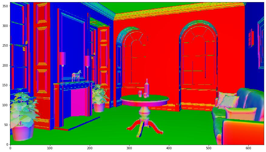
# Render
lm.asset('film_output', 'film::bitmap', {
    'w': 640,
    'h': 360
})
lm.render('renderer::raycast', {
    'output': lm.asset('film_output')
})
img = np.copy(lm.buffer(lm.asset('film_output')))

# Visualize
f = plt.figure(figsize=(15,15))
ax = f.add_subplot(111)
ax.imshow(np.clip(np.power(img,1/2.2),0,1), origin='lower')
plt.show()

[I|1.232|48@assets ] Loading asset [name='film_output']
[I|1.242|151@user  ] Starting render [name='renderer::raycast']