Rendering with path tracing
This example describes how to render the scene with path tracing. Path tracing is a rendering technique based on Monte Carlo method and notably one of the most basic (yet practical) rendering algorithms taking global illumination into account. Our framework implements path tracing as renderer::pt renderer.
The use of the renderer is straightforward; we just need to specify renderer::pt with lm::render() function with some renderer-specific parameters. Thanks to the modular design of the framework, the most of the code can be the same as Raycasting a scene with OBJ models.
[1]:
import os
import numpy as np
import imageio
%matplotlib inline
import matplotlib.pyplot as plt
import lmfunctest as ft
import lightmetrica as lm
%load_ext lightmetrica_jupyter
[2]:
lm.init()
lm.log.init('logger::jupyter')
lm.progress.init('progress::jupyter')
lm.info()
[I|0.000|114@user ] Lightmetrica -- Version 3.0.0 (rev. fe30e7c) Linux x64
[3]:
# Film for the rendered image
lm.asset('film1', 'film::bitmap', {
    'w': 1920,
    'h': 1080
})

# Pinhole camera
lm.asset('camera1', 'camera::pinhole', {
    'position': [5.101118, 1.083746, -2.756308],
    'center': [4.167568, 1.078925, -2.397892],
    'up': [0,1,0],
    'vfov': 43.001194
})

# OBJ model
lm.asset('obj1', 'model::wavefrontobj', {
    'path': os.path.join(ft.env.scene_path, 'fireplace_room/fireplace_room.obj')
})
[I|0.013|48@assets ] Loading asset [name='film1']
[I|0.105|48@assets ] Loading asset [name='camera1']
[I|0.105|48@assets ] Loading asset [name='obj1']
[I|0.105|29@objload]   Loading OBJ file [path='fireplace_room.obj']
[I|0.105|169@objloa]   Loading MTL file [path='fireplace_room.mtl']
[I|0.106|44@texture]   Loading texture [path='wood.ppm']
[I|0.216|44@texture]   Loading texture [path='leaf.ppm']
[I|0.220|44@texture]   Loading texture [path='picture8.ppm']
[I|0.264|44@texture]   Loading texture [path='wood5.ppm']
[3]:
'$.assets.obj1'
[4]:
# Camera
lm.primitive(lm.identity(), {
    'camera': lm.asset('camera1')
})

# Create primitives from model asset
lm.primitive(lm.identity(), {
    'model': lm.asset('obj1')
})
[5]:
lm.build('accel::sahbvh', {})
lm.render('renderer::pt', {
    'output': lm.asset('film1'),
    'spp': 10,
    'maxLength': 20
})
[I|0.760|246@scene ] Building acceleration structure [name='accel::sahbvh']
[I|0.761|131@accel_]   Flattening scene
[I|0.794|261@accel_]   Building
[I|1.679|151@user  ] Starting render [name='renderer::pt']
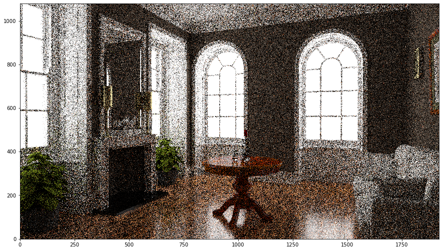
[6]:
img = np.copy(lm.buffer(lm.asset('film1')))
f = plt.figure(figsize=(15,15))
ax = f.add_subplot(111)
ax.imshow(np.clip(np.power(img,1/2.2),0,1), origin='lower')
plt.show()