Rendering quad
This example describes how to render a simple scene containing a quad represented by two triangles. The code starts again with lm::init() function.
[1]:
import numpy as np
import imageio
%matplotlib inline
import matplotlib.pyplot as plt
import lmfunctest as ft
import lightmetrica as lm
%load_ext lightmetrica_jupyter
[2]:
lm.init()
lm.log.init('logger::jupyter')
lm.progress.init('progress::jupyter')
lm.info()
[I|0.000|114@user ] Lightmetrica -- Version 3.0.0 (rev. fe30e7c) Linux x64
Similarly we define the assets. In addition to film, we define camera, mesh, and material. Although the types of assets are different, we can use consistent interface to define the assets. Here we prepare for a pinhole camera (camera::pinhole), a raw mesh (mesh::raw), and a diffuse material (material::diffuse) with the corrsponding parameters. Please refer to Built-in component reference for the detailed description of the parameters.
[3]:
# Film for the rendered image
lm.asset('film1', 'film::bitmap', {
    'w': 1920,
    'h': 1080
})

# Pinhole camera
lm.asset('camera1', 'camera::pinhole', {
    'position': [0,0,5],
    'center': [0,0,0],
    'up': [0,1,0],
    'vfov': 30
})

# Load mesh with raw vertex data
lm.asset('mesh1', 'mesh::raw', {
    'ps': [-1,-1,-1,1,-1,-1,1,1,-1,-1,1,-1],
    'ns': [0,0,1],
    'ts': [0,0,1,0,1,1,0,1],
    'fs': {
        'p': [0,1,2,0,2,3],
        'n': [0,0,0,0,0,0],
        't': [0,1,2,0,2,3]
    }
})

# Material
lm.asset('material1', 'material::diffuse', {
    'Kd': [1,1,1]
})
[I|0.014|48@assets ] Loading asset [name='film1']
[I|0.102|48@assets ] Loading asset [name='camera1']
[I|0.105|48@assets ] Loading asset [name='mesh1']
[I|0.106|48@assets ] Loading asset [name='material1']
[3]:
'$.assets.material1'
The scene of Lightmetrica is defined by a set of primitives. A primitive specifies an object inside the scene by associating geometries and materials with transformation. We can define a primitive by lm::primitive() function where we specifies transformation matrix and associating assets as arguments.
In this example we define two pritimives; one for camera and the other for quad mesh with diffuse material. Transformation is given by 4x4 matrix. Here we specified identify matrix meaning no transformation.
Note
Specifically, the scene is represented by a scene graph, a directed acyclic graph representing spatial structure and attributes of the scene. Each node of the scene graph describes either a primitive or a pritmive group. We provide a set of APIs to manipulate the structure of scene graph for advanced usage like instancing. For detail, please refer to TODO.
[4]:
# Camera
lm.primitive(lm.identity(), {
    'camera': lm.asset('camera1')
})

# Mesh
lm.primitive(lm.identity(), {
    'mesh': lm.asset('mesh1'),
    'material': lm.asset('material1')
})
This example used renderer::raycast for rendering.
This renderer internally uses acceleration structure for ray-scene intersections.
The acceleration structure can be given by lm::build() function. In this example we used accel::sahbvh.
[5]:
lm.build('accel::sahbvh', {})
lm.render('renderer::raycast', {
    'output': lm.asset('film1'),
    'color': [0,0,0]
})
[I|0.129|246@scene ] Building acceleration structure [name='accel::sahbvh']
[I|0.129|131@accel_]   Flattening scene
[I|0.129|261@accel_]   Building
[I|0.130|151@user  ] Starting render [name='renderer::raycast']
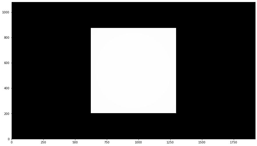
[6]:
img = np.copy(lm.buffer(lm.asset('film1')))
f = plt.figure(figsize=(15,15))
ax = f.add_subplot(111)
ax.imshow(np.clip(np.power(img,1/2.2),0,1), origin='lower')
plt.show()